Adding elevation to DOC track dataset
I don’t know if this is interesting to anyone, but on Friday and for an extra hour or two in the weekend, I was playing around with calculating an elevation profile for walking tracks in NZ.
I started with a dataset from data.govt.nz from the Department of Conservation (which for AU is responsible for walking tracks and facilities at a national level - basically all the national parks, and big walks - local councils take care of smaller parks, tracks etc). That dataset has just over 3,000 records, including a track name, distance in meters, and a path comprised of X,Y points.
For the elevation, I grabbed a dataset from LINZ (Land Information NZ), who maintain topographical map coverage of NZ. The topomaps have lots of detail on them, but I was interested in the contours. Contours are shapes that indicate elevation on a map. Contour lines that are closer together indicate steeper ground, and farther apart, a gentler climb. For the Topo50 map series in NZ, a contour line indicates an altitude gain or loss of 20m. Every 100m, a contour line is displayed as a bolder line with a label indicating the altitude. In the dataset I downloaded from LINZ, contours are represented as polygons. This dataset was reasonably small - 1.8gb compressed. I investigated a digital elevation model, or DEM. This is basically a giant dataset of points, associated with an altitude. Usually, this data is collected from air or spare using LiDAR, which is basically bouncing a laser beam off the ground and measuring the distance. In NZ, LiDAR coverage is still limited to around the main centres. I am going to investigate this more, since there are a couple of 8-meter resolution DEM datasets that I might be able to use - these are derived from the contour lines anyway though, rather than something as precise as LiDAR.
I set up a new PostGIS database, and imported the two datasets, which I had
downloaded as shapefiles, using GDAL, in particular, ogr2ogr. GDAL is to
geospatial data what ImageMagick is to image data, and is great and converting
between formats. Once I had imported this data, I had two tables, doc_tracks,
and nz_contours_topo_150k.
I then did a bit of googling, and immediately found a query that did almost literally exactly what I wanted - took an existing line shape, and existing elevation data, and matched one with the other to create a new line shape with elevation (Z axis) added:
WITH
    sequenced_points AS (
        SELECT description, status, length_over_ground, object_type, equipment,
               mln_seq,
               pts.path[1] AS elem_seq,
               pts.path[2] AS pnt_seq,
               pts.geom AS geom
        FROM (
            SELECT descriptio as description, status, shape_leng as length_over_ground, object_typ as object_type, equipment,
                   ROW_NUMBER() OVER() AS mln_seq,
                   (ST_DumpPoints(wkb_geometry)).*
            FROM doc_tracks
        ) AS pts
    )

SELECT DISTINCT
       description, status, length_over_ground, object_type, equipment,
       ST_MakeLine(st_setsrid(ST_MakePoint(ST_X(sequenced_points.geom), ST_Y(sequenced_points.geom), q.elevation), 2193)) OVER(PARTITION BY sequenced_points.mln_seq, sequenced_points.elem_seq ORDER BY sequenced_points.elem_seq) AS geom
FROM sequenced_points
JOIN LATERAL (
    SELECT elevation
    FROM nz_contours_topo_150k
    ORDER BY wkb_geometry <-> sequenced_points.geom
    LIMIT 1
) AS q
ON true;
This query isn’t too hard to parse, but uses a few techniques that are unusual for my normal webapp CRUD queries. It uses a lateral join, common table expression, and partitioning. The original answer did not have a call to ST_SetSRID, which I added, since otherwise the point is constructed without an SRID, which means any mapping software will not know how to display it. The SRID of both datasets I imported is 2193, which is the NZTM projection used throughout NZ. I could have reprojected either, or both datasets to ‘regular’ latitudes and longitudes, WGS84 or 4326, but this would distort the track paths, which I needed to keep quite precise.
This query worked, but was incredibly slow. I also found it hard to run for just one track at a time, because in the CTE, the first thing it does is break the track path into individual points. So putting a LIMIT clause on that just returned part of a track.
I stated looking at how to speed this up. The first thing I did, was add indices to the geospatial columns:
-- Create an index on the contour line polygon geometry
create index nz_contours_topo_150k_geo on nz_contours_topo_150k using gist (wkb_geometry);

-- Create an index on the doc track geometry
create index doc_tracks_geo on doc_tracks using gist (wkb_geometry);
This didn’t really help. The index nz_contours_topo_150k also took a suspiciously short amount of time. Almost like it didn’t do anything at all…
The next thing I did was move the preprocessing of the track lines into a new table. This meant my elevation-adding query got much simpler, since it didn’t need to partition any more:
create table doc_track_points as (
 SELECT tracks.descriptio as description,
        	   tracks.object_typ as track_grade,
               mln_seq,
               tracks.path[1] AS elem_seq,
               tracks.path[2] AS pnt_seq,
               tracks.geom AS geom
        FROM (
            SELECT descriptio, -- <some_other_column>,
                   object_typ,
                   ROW_NUMBER() OVER() AS mln_seq,
                   (ST_DumpPoints(wkb_geometry)).*
            FROM doc_tracks
        ) AS tracks);
create index doc_track_points_seq_idx on doc_track_points (mln_seq, elem_seq);
create index doc_track_points_geom_idx on doc_track_points using gist (geom);
With the track points in their own table, I could filter the rows to just return points for a particular track:
SELECT
       dtp.description, dtp.track_grade,
       st_setsrid(st_makepoint(st_x(dtp.geom), st_y(dtp.geom), q.elevation), 2193) as geom
from doc_track_points dtp
JOIN LATERAL (
    SELECT elevation
    FROM nz_contours_topo_150k
    ORDER BY wkb_geometry <-> dtp.geom
    LIMIT 1
) AS q
ON true
WHERE dtp.description='Upper Fenian/Fenian Gold/Adams Flat Trk';
This track has 167 points along it’s route - not a tonne. It took 6 minutes to add elevation to it. It wouldn’t have been impossible just to have this run and generate all the data, but I still felt it should be faster than this for that number of points. Because I was operating on one point at a time, and adding the elevation to it, I would still need to post-process that table’s data back into an actual line at some point as well.
The next thing I did was start running EXPLAIN ANALYZE on the query. Prefixing a query with EXPLAIN (ANALYZE, COSTS, VERBOSE, BUFFERS, FORMAT JSON) generates a JSON output that can be pasted into a visualisation tool like https://explain.depesz.com/ to visualise where the query is spending it’s time.

Using this tool, I could see that even though the correct indexes were being used, nearly the entire query time was being spent matching contour polygons to track points. This isn’t terribly surprising, since this is where the actual geospatial calculation is happening - everything else is mostly just a straight operator-based query.
Since indexes were already being used, I was a bit stuck here, but I had a suspicion - while there are well-established mathmatical formula for finding the nearest point on a polygon to a point (and in fact this is how Postgis is matching the polygon to the point internally), it’s still a potentially expensive calculation that needs to be done. I wondered whether the query performance would be improved if I “exploded” the contour lines out into their respective points, indexed these, and then matched on individual points, rather than a whole polygon. I particularly suspected that indexing these points would result in an efficiency gain, because PostGIS geospatial indexes are very much optimised for finding the nearest point to another point.
So, I used ST_DumpPoints as I had for getting the points from a track line, to dump out the points comprising a contour polygon, into a table:
create table contour_line_points as (
	select nctk.geom as wkb_geometry,
		   nctk.elevation
	from (
		select elevation,
			   (ST_DumpPoints(wkb_geometry)).*
		from nz_contours_topo_150k
	) as nctk
);
This table took a few minutes to generate - not bad.
I then added an index to this table. This took a very long time - about 13 hours - but I wasn’t too worried. I had expected it to be slow, and essentially once the index was built, I wouldn’t have to rebuild it unless I change the underlying data. I probably could also tune some Postgres settings like maintenance_work_mem to try and speed this up.
create index contour_line_points_geom on contour_line_points using gist (wkb_geometry);
Now I ran the query for resolving the track points above, but swapped out the table name - contour_line_points instead of nz_contours_topo_150k. I could leave the operator the same, because the operator already knows how to handle different types of geospatial data - I’ve just switched it from matching a polygon to a point, to a point to a point.
Now when I ran the same query for that single track with 167 points, it took around 250ms. A great improvement! It was such a good improvement that I rolled my query back to the original version. I preferred this version because it didn’t require me to pre-process the track lines into points then have to post-process them back into a line - I could just take in the 2D line, and return the 3D line with elevation added. I ran it, and off it went. It still took a couple of hours to run, so I prefixed the query with CREATE TABLE doc_tracks_elevation AS. This meant the result of the query was written to a table so that I could quickly query data from the returned dataset (using CREATE MATERIALIZED VIEW AS here would have been better, since I could refresh the view easily, but I didn’t think of it at the time). The query for generating this table I ended up with was:
create table doc_tracks_elevation as
WITH
    sequenced_points AS (
        SELECT description, status, length_over_ground, object_type, equipment,
               mln_seq,
               pts.path[1] AS elem_seq,
               pts.path[2] AS pnt_seq,
               pts.geom AS geom
        FROM (
            SELECT descriptio as description, status, shape_leng as length_over_ground, object_typ as object_type, equipment,
                   ROW_NUMBER() OVER() AS mln_seq,
                   (ST_DumpPoints(wkb_geometry)).*
            FROM doc_tracks
        ) AS pts
    )

SELECT DISTINCT
       description, status, length_over_ground, object_type, equipment,
       ST_MakeLine(st_setsrid(ST_MakePoint(ST_X(sequenced_points.geom), ST_Y(sequenced_points.geom), q.elevation), 2193)) OVER(PARTITION BY sequenced_points.mln_seq, sequenced_points.elem_seq ORDER BY sequenced_points.elem_seq) AS geom
FROM sequenced_points
JOIN LATERAL (
    SELECT elevation
    FROM contour_line_points
    ORDER BY wkb_geometry <-> sequenced_points.geom
    LIMIT 1
) AS q
ON true;
A little while later (about an hour), and I have 4,850 tracks with elevation. Why is the number higher than the original? Well, that’s a good question. I believe it is because some tracks, for whatever reason, have more than one line associated with them. This could be because of a river or tidal crossing, where DOC have represented the track as two segments rather than one continuous line. Because of the way the ST_DumpPoints and partitition works, it returns a distinct row per line, rather than a multiline. At the moment, this is fine for me to continue to start to visualise this data. In the future, I will post-process these line shapes back into a multiline by matching against the track description and/or objectid.
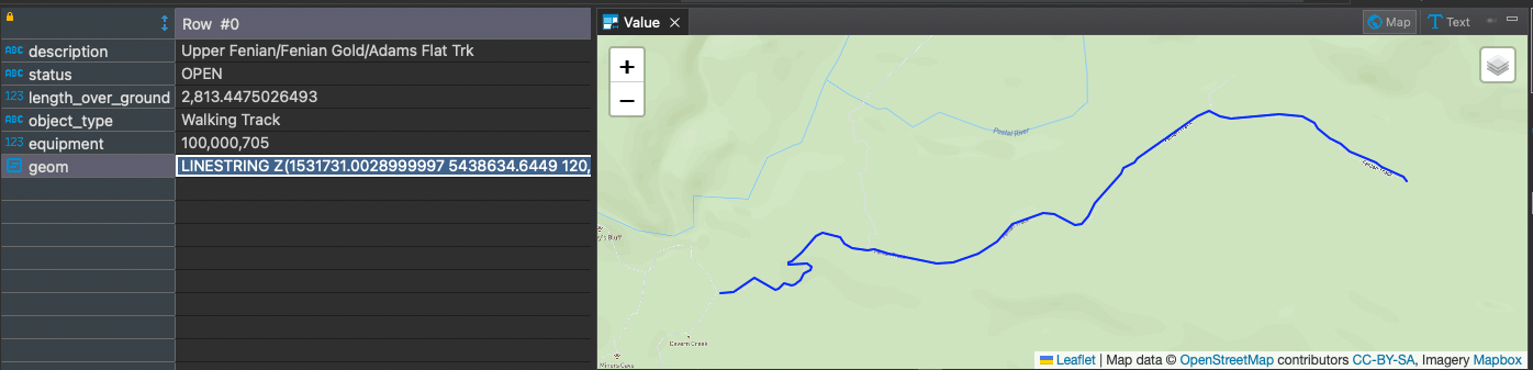
Selecting a single track’s information is as fast as I would expect it to be, since I don’t need to recalculate each time I want the elevation of a track:
select * from doc_tracks_elevation where description='Upper Fenian/Fenian Gold/Adams Flat Trk';
=> Time: 20.296 ms
Now that I have calculated the basic elevation data, I’ve got some work to do to start visualising this data. I’ve also identified some optimisations in my current process I’d like to put in place.
For visualisation, I plan to generate a JSON file for each track, as well as a manifest that can be used for an autocomplete search. The idea would be that someone can search for a track, which then fetches the JSON containing the 3D track route. I would use the elevation points from this route to show a graph of the elevation over distance, as well as the route itself. I may experiment with web mapping libraries that support 3D, like Mapbox, to show the track against a 3D terrain layer. With the Z axis defined, I can also generate the actual travel distance for each track, rather than just distance over ground that comes from the route.
For the data processing stage, I would like to switch to using a DEM - probably the 8m derived DEM from contours. While exploding the contour points has yielded sufficient results, it’s not very high resolution. As far as I know, ST_DumpPoints just dumps the ‘corners’ of polygons, and not the intermediate points. That means that I might not be finding the correct elevation for a track point - it all depends on the orientation of nearby contours. Using a DEM with a 8m grid means that I can return more accurate elevation. I also would like to investigate which tracks have multiple lines, and ensure that I can post-process these back into their original form. I would also like to look at augmenting the track path data with some statistics - things like gain/drop, as well as the actual track distance as I mentioned above. Finally, to assist the visualiation, I would like to add marker points to the data every kilometer across the ground, and kilometer based on track distance. This would help to break the track path into segments to allow users to have a reference point for a particular area of climb or descent.